Convolutional Neural Networks (CNNs / ConvNets)
Convolutional neural networks as very similar to the ordinary feed-forward neural networks. They differ in the sense that CNNs assume explicitly that the inputs are images, which enables us to encode specific properties in the architecture to recognize certain patterns in the images. The CNNs make use of spatial nature of the data. It means, CNNs perceive the objects similar to our perception of different objects in nature. For example, we recognize various objects by their shapes, size and colors. These objects are combinations of edges, corners, color patches, etc. CNNs can use a variety of detectors (such as edge detectors, corner detectors) to interpret images. These detectors are called filters or kernels. The mathematical operator that takes an image and a filter as input and produces a filtered output (e.g. edges, corners, etc. ) is called convolution.
 Learned features in a CNN. [Image Source]
CNNs Architecture
Convolutional Neural Networks have a different architecture than regular Neural Networks. CNNs are organized in 3 dimensions (width, height and depth). Also, Unlike ordinary neural networks that each neuron in one layer is connected to all the neurons in the next layer, in a CNN, only a small number of the neurons in the current layer connects to neurons in the next layer.
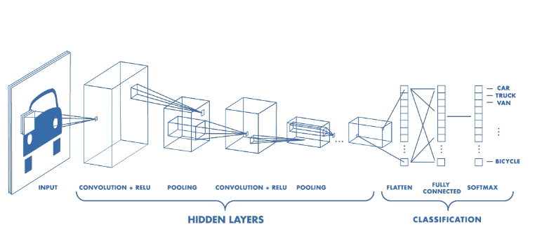 Architecture of a CNN. [Image Source]
ConvNets have three types of layers: Convolutional Layer, Pooling Layer and Fully-Connected Layer. By stacking these layers we can construct a convolutional neural network.
Convolutional Layer
Convolutional layer applies a convolution operator on the input data using a filter and produces an output that is called feature map. The purpose of the convolution operation is to extract the high-level features such as edges, from the input image. The first ConvLayer is captures the Low-Level features such as edges, color, orientation, etc. Adding more layers enables the architecture to adapt to the high-level features as well, giving us a network which has the wholesome understanding of images in the dataset.
We execute a convolution by sliding the filter over the input. At every location, an element-wise matrix multiplication is performed and sums the result onto the feature map.
 Left: the filter slides over the input. Right: the result is summed and added to the feature map. [Image Source]
The example above was a convolution operation shown in 2D using a 3x3 filter. But in reality these convolutions are performed in 3D because an image is represented as a 3D matrix with dimensions of width, height and depth, where depth corresponds to color channels (RGB). Therefore, a convolution filter covers the entire depth of its input so it must be 3D as well.
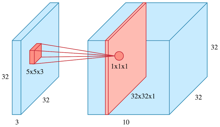 The filter of size 5x5x3 slides over the volume of input. [Image Source]
We perform many convolutions on our input, where each convolution operation uses a different filter. This results in different feature maps. At the end, we stack all of these feature maps together and form the final output of the convolution layer.
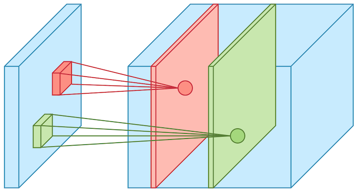 Example of two filters (green and red) over the volume of input. [Image Source]
In order to make our output non-linear, we pass the result of the convolution operation through an activation function (usually ReLU). Thus, the values in the final feature maps are not actually the sums, but the ReLU function applied to them.
Stride and Padding
Stride is the size of the step we move the convolution filter at each step. The default value of the stride is 1.
 Stride with value of 1. [Image Source]
If we increase the size of stride the feature map will get smaller. The figure below demonstrates a stride of 2.
 Stride with value of 2. [Image Source]
We can see that the size of the feature map feature is reduced in dimensionality as compared to the input. If we want to prevent the feature map from shrinking, we apply padding to surround the input with zeros.
 Stride = 1 with padding = 1. [Image Source]
Pooling Layer
After a convolution layer we usually perform pooling to reduce the dimensionality. This allows us to reduce the number of parameters, which both shortens the training time and prevents overfitting. Pooling layers downsample each feature map independently, reducing the width and height and keeping the depth intact. max pooling is the most common types of pooling, which takes the maximum value in each window. Pooling does not have any parameters. It just decreases the size of the feature map while at the same time keeping the important information (i.e. dominant features).
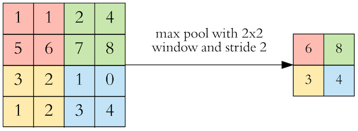 Max pooling takes the largest value. [Image Source]
Hyperparameters
When using ConvNets, there are certain hyperparameters that we need to determine.
- Filter size (kernel size): 3x3 filter are very common, but 5x5 and 7x7 are also used depending on the application.
- Filter count: How many filters do we want to use. It’s a power of two anywhere between 32 and 1024. The more filters, the more powerful model. However, there is a possibility of overfitting due to large amount of parameters. Therefore, we usually start off with a small number of filters at the initial layers, and gradually increase the count as we go deeper into the network.
- Stride: The common stride value is 1
- Padding:
Fully Connected Layer (FC Layer)
We often have a couple of fully connected layers after convolution and pooling layers. Fully connected layers work as a classifier on top of these learned features. The last fully connected layer outputs a N dimensional vector where N is the number of classes. For example, for a digit classification CNN, N would be 10 since we have 10 digits. Please note that the output of both convolution and pooling layers are 3D volumes, but a fully connected layer only accepts a 1D vector of numbers. Therefore, we flatten the 3D volume, meaning we convert the 3D volume into 1D vector.
 A CNN to classify handwritten digits. [Image Source]
Training ConvNets
Training CNNs is the same as ordinary neural networks. We apply backpropagation with gradient descent. For reading about training neural networks please see here.
ConvNets Architectures
This section is adopted from Stanford University course here. Convolutional Networks are often made up of only three layer types: CONV, POOL (i.e. Max Pooling), FC. Therefore, the most common architecture pattern is as follows:
INPUT -> [[CONV -> RELU]*N -> POOL?]*M -> [FC -> RELU]*K -> FC
where the * indicates repetition, and the POOL? indicates an optional pooling layer. Moreover, N >= 0 (and usually N <= 3), M >= 0, K >= 0 (and usually K < 3).
There are several architectures of CNNs available that are very popular:
- LeNet
- AlexNet
- ZF Net
- GoogLeNet
- VGGNet
- ResNet
Implementation
As a practice, I created a ConvNet to classify latex symbols. Particularly, I download the HASY data set of handwritten symbols from here. It includes 369 classes including Arabic numerals and Latin characters. I split the dataset into 80% train, 20% test and trained the CNN on training set. For training I used the Google colab utilizing GPU computations. Here's the link to colab notebook. I got the accuracy of 81.75% on the test set. It definitely has room to be improved. The architecture of the CNN is as follows:
Model: "sequential"
_________________________________________________________________
Layer (type)                 Output Shape              Param #
=================================================================
conv2d (Conv2D)              (None, 32, 32, 128)       1280
_________________________________________________________________
conv2d_1 (Conv2D)            (None, 32, 32, 128)       147584
_________________________________________________________________
max_pooling2d (MaxPooling2D) (None, 16, 16, 128)       0
_________________________________________________________________
dropout (Dropout)            (None, 16, 16, 128)       0
_________________________________________________________________
conv2d_2 (Conv2D)            (None, 16, 16, 128)       409728
_________________________________________________________________
max_pooling2d_1 (MaxPooling2 (None, 8, 8, 128)         0
_________________________________________________________________
flatten (Flatten)            (None, 8192)              0
_________________________________________________________________
dense (Dense)                (None, 128)               1048704
_________________________________________________________________
dropout_1 (Dropout)          (None, 128)               0
_________________________________________________________________
dense_1 (Dense)              (None, 128)               16512
_________________________________________________________________
dense_2 (Dense)              (None, 369)               47601
=================================================================
Total params: 1,671,409
Trainable params: 1,671,409
Non-trainable params: 0
In order to make this project more interesting, I converted the python-keras model into a Tenserflowjs model, then developed a simple Web application using Javascript, loaded the model and used it for predicting latex symbol by drawing symbols in a canvas. Here's the GitHub link for the Web app. Below is a snapshot of how it works:

# Create id2latex and latex2id maps
symbol_file_name = 'symbols.csv'
data_file_name   = 'hasy-data-labels.csv'
id2latex,latex2id = load_symbols(symbol_file_name)
data,labels = load_data(data_file_name,latex2id)

# Randomly pick an example and display it
sample = 83643
img = Image.fromarray(data[sample])
plt.imshow(img)
print(id2latex[labels[sample]])

# Split the data into train and test sets
train_data,test_data,train_labels,test_labels = train_test_split(data,labels,test_size=0.2)

# Normalizing train and test data
normalized_train_data = np.asarray(train_data)/255.0
normalized_test_data = np.asarray(test_data)/255.0

# One-hot encoding of labels for train and test datasets
encoded_train_labels = np.array(keras.utils.to_categorical(train_labels))
encoded_test_labels = np.array(keras.utils.to_categorical(test_labels))

# Reshaping train and test sets, i.e. changing from (32, 32) to (32, 32, 1)
normalized_train_data = normalized_train_data.reshape(-1,32,32,1)
normalized_test_data = normalized_test_data.reshape(-1,32,32,1)

print('Input shape = {}'.format(normalized_train_data.shape[1:]))
print('Number of classes =  {}'.format(encoded_train_labels.shape[1]))

# Define intial variables
input_features = normalized_train_data.shape[1]
n_classes = encoded_train_labels.shape[1]
batch_size = 128
epochs = 15

# Define the CNN model

model = Sequential()
model.add(Conv2D(128, (3,3), activation='relu', padding='same', input_shape=(input_features,input_features,1)))
model.add(Conv2D(128,(3,3), activation='relu', padding='same'))
model.add(MaxPooling2D((2,2)))
model.add(Dropout(0.5))
model.add(Conv2D(128,(5,5), activation='relu', padding='same'))
model.add(MaxPooling2D((2,2)))
model.add(Flatten())
model.add(Dense(128, activation='relu'))
model.add(Dropout(0.5))
model.add(Dense(128, activation='relu'))
model.add(Dense(n_classes, activation='softmax'))

model.summary()

# Train the model
model.compile(optimizer='adam', loss='categorical_crossentropy', metrics=['accuracy'])
model.fit(normalized_train_data,encoded_train_labels, batch_size=batch_size, epochs=epochs, verbose=1, validation_data=(normalized_test_data,encoded_test_labels))
Train on 134586 samples, validate on 33647 samples
Epoch 1/15
134586/134586 [==============================] - 55s 412us/sample - loss: 2.9116 - accuracy: 0.3689 - val_loss: 1.1192 - val_accuracy: 0.6942
Epoch 2/15
134586/134586 [==============================] - 48s 357us/sample - loss: 1.6461 - accuracy: 0.5727 - val_loss: 0.8604 - val_accuracy: 0.7529
Epoch 3/15
134586/134586 [==============================] - 48s 356us/sample - loss: 1.3399 - accuracy: 0.6383 - val_loss: 0.7842 - val_accuracy: 0.7749
Epoch 4/15
134586/134586 [==============================] - 48s 356us/sample - loss: 1.1756 - accuracy: 0.6739 - val_loss: 0.7115 - val_accuracy: 0.7893
Epoch 5/15
134586/134586 [==============================] - 48s 354us/sample - loss: 1.0635 - accuracy: 0.7013 - val_loss: 0.7017 - val_accuracy: 0.7889
Epoch 6/15
134586/134586 [==============================] - 48s 355us/sample - loss: 0.9863 - accuracy: 0.7164 - val_loss: 0.6497 - val_accuracy: 0.8052
Epoch 7/15
134586/134586 [==============================] - 48s 354us/sample - loss: 0.9254 - accuracy: 0.7306 - val_loss: 0.6536 - val_accuracy: 0.8029
Epoch 8/15
134586/134586 [==============================] - 48s 356us/sample - loss: 0.8730 - accuracy: 0.7439 - val_loss: 0.6280 - val_accuracy: 0.8069
Epoch 9/15
134586/134586 [==============================] - 48s 354us/sample - loss: 0.8305 - accuracy: 0.7530 - val_loss: 0.6123 - val_accuracy: 0.8149
Epoch 10/15
134586/134586 [==============================] - 48s 356us/sample - loss: 0.7942 - accuracy: 0.7614 - val_loss: 0.6133 - val_accuracy: 0.8117
Epoch 11/15
134586/134586 [==============================] - 48s 354us/sample - loss: 0.7660 - accuracy: 0.7686 - val_loss: 0.5940 - val_accuracy: 0.8172
Epoch 12/15
134586/134586 [==============================] - 48s 355us/sample - loss: 0.7425 - accuracy: 0.7735 - val_loss: 0.5928 - val_accuracy: 0.8185
Epoch 13/15
134586/134586 [==============================] - 48s 355us/sample - loss: 0.7229 - accuracy: 0.7775 - val_loss: 0.5971 - val_accuracy: 0.8167
Epoch 14/15
134586/134586 [==============================] - 48s 355us/sample - loss: 0.7039 - accuracy: 0.7822 - val_loss: 0.5893 - val_accuracy: 0.8198
Epoch 15/15
134586/134586 [==============================] - 48s 355us/sample - loss: 0.6867 - accuracy: 0.7867 - val_loss: 0.5890 - val_accuracy: 0.8175
score = model.evaluate(normalized_test_data, encoded_test_labels, verbose=0)
print('Test loss: {:.3f}'.format(score[0]))
print('Test accuracy: {:.2f}%'.format(score[1] * 100))
Test loss: 0.589
Test accuracy: 81.75%