Classification
Classification is a learning algorithm that determines which discrete category a new example (instance) belongs, given a set of training instances $X$ with their observed categories $Y$. Binary classification is a classification task where $Y$ has two possible values $0,1$. If $Y$ has more than two possible values, it is called a multi-class classification.
Can we use Linear Regression for classification problems?
Thare are two main issues with using linear regression for classification:
Linear regression outputs values for $Y$ that can be much larger than 1 or much lower than 0, but our classes are 0 and 1.
Our hypothesis or prediction rule can change each time a new training example arrives, which shouldn't. Instead, we should be able to use the learned hypothesis to make correct predictions for the data we haven't seen before.

Naive Bayes
If we have consider Naive Bayes assumption, then we have: $$P(X_1\cdots X_d|Y)=\prod_{i=1}^{d}P(X_i|Y)$$
We also assume parametric form for $P(X_i|Y)$ and $P(Y)$. Then, we use MLE or MAP to estimate the parameters.
At last, Naive Bayes classifier for a $X^{new} = <X_1,X_2,\cdots X_d>$ is:
$$Y^{new} =\underset{y}{\arg\max}\quad P(Y=y_k)\prod_i P(X^{new}_i|Y=y_K)$$
Generative vs Discriminative Classifiers
Training a classifier involves estimating $P(Y|X)$.
i. Generative classifiers (e.g. Naive Bayes):
- Assume some functional form for $P(X,Y)$, i.e. $P(X|Y)$ and $P(Y)$
- Estimate parameters of $P(X|Y)$, $P(Y)$ directly from training data
- $\underset{y}{\arg\max}\quad P(X|Y)P(Y)= \underset{y}{\arg\max}\quad P(Y|X)$
Question: Can we learn the $P(Y|X)$ directly from data? Or better yet, can we learn decision boundary directly?
ii. Discriminative classifiers (e.g. Logistic Regression):
- Assume some functional form for $P(Y|X)$ or for the decision boundary
- Estimate parameters of $P(Y|X)$ directly from training data
Logistic Regression
Logistic regression is a classification method for binary classification problems, where input $X$ is a vector of discrete or real-valued variables and $Y$ is discrete (boolean valued). The idea is to learn $P(Y|X)$ directly from observed data.
Let's consider learning $f:X\rightarrow Y$ where,
- $X$ is a vector of real-valued features, $<X_1,\cdots,X_n>$
- $Y$ is boolean
- Assume all $X_i$ are conditionally independent given $Y$
- Assume $P(X_i|Y=y_k) \sim N(\mu_{ik},\sigma_i)$
- Assume $P(Y) \sim $ Bernoulli($\pi$)
What does this imply about the form of $P(Y|X)$?
$$P(Y=0|X=<X_1,\cdots,X_n>)=\frac{1}{1+exp(w_0+\sum_{i}w_iX_i)}$$
$$P(Y=1|X) = 1 - P(Y=1|X) = \frac{\exp(w_0+\sum_{i=1}^{n}w_iX_i)}{1+\exp(w_0+\sum_{i=1}^{n}w_iX_i)} $$
$$g(z)=\frac{1}{1+e^{-z}}$$
 Fig1. Sigmoid Function
Logistic Regression is Linear
The reason that logistic regression is linear is that, the outcome is a linear combinations of the inputs and parameters.
$$\frac{P(Y=1|X)}{P(Y=0|X)} = \exp(w_0+\sum_{i=1}^{n}w_iX_i)$$
which implies:
$$\ln\frac{P(Y=1|X)}{P(Y=0|X)} = w_0+\sum_{i=1}^{n}w_iX_i$$
where $w_0+\sum_{i=1}^{n}w_iX_i$ is the linear classification rule.
Decision Boundary
Since logistic regression prediction function returns a probability between 0 and 1, in order to predict which class this data belongs we need to set a threshold. For each data point, if the estimated probability is above this threshold, we classify the point into class 1, and if it's below the threshold, we classify the point into class 2.
If $P(Y=1|X)\geq0.5$, class $=1$, and if $P(Y=1|X)<0.5$, class $=0$.
Training Logistic Regression: MLCE
We have a collection of training data $D = \{<X^1,Y^1>,\cdots,<X^M,Y^M>\}$. We need to find the parameters $\mathbf{w}=<w_0,\cdots,w_n>$ that maximize the conditional likelihood of the training data.
Data likelihood $=\prod_j P(<X^j,Y^j>|\mathbf{w})$, thus data conditional likelihood $=\prod_j P(Y^j|X^j,\mathbf{w})$.
therefore, $$W_{MLCE}=\underset{\mathbf{w}}{\arg\max}\prod_j P(Y^j|X^j,\mathbf{w})$$
In order to make arithmetic easier, we work with the conditional log likelihood. Additionally, we know that maximizing a function is equivalent to minimizing the negative of the function. Therefore, we convert our problem to a minimization problem and apply the Gradient Descent algorithm to find the minimum. $$ \begin{aligned} W_{MLCE}&=\underset{\mathbf{w}}{\arg\max}\quad \ln \prod_j P(Y^j|X^j,\mathbf{w}) = \sum_j \ln P(Y^j|X^j,\mathbf{w})\\ &=\underset{W}{\arg\max}\quad\sum_j \ln P(Y^j|X^j,\mathbf{w})\\ &=\underset{W}{\arg\min}\quad -\sum_j \ln P(Y^j|X^j,\mathbf{w}) \end{aligned} $$
if $J(\mathbf{w})=-\sum_j \ln P(Y^j|X^j,\mathbf{w})$, then we have:
$$\begin{aligned} J(\mathbf{w})&=-\sum_j \left [ Y^j \ln P(Y^j=1|X^j,\mathbf{w}) + (1-Y^j) \ln P(Y^j=0|X^j,\mathbf{w})\right ]\\ &=-\sum_j \left[ Y^j(w_0+\sum_iw_iX_i^j)-\ln(1+\exp(w_0+\sum_iw_iX_i^j))\right ] \end{aligned} $$$J(\mathbf{w})$ is a convex function, so we can always find global minimum. There is no closed-form solution to minimize it. However, we can use gradient descent algorithm to find the minimum.
Gradient Descent algorithm for Logistic Regression
- Compute the gradient of $J_D(\mathbf{w})$ over the entire training set $D$: $$\nabla J_D(\mathbf{w}) = \left [\frac{\partial J_D(\mathbf{w})}{\partial w_0},\cdots \frac{\partial J_D(\mathbf{w})}{\partial w_n} \right]$$
$$\frac{\partial J_D(\mathbf{w})}{\partial w_i}=\sum_{j=1}^{M}X_i^j\left[Y^j-\hat{P}(Y^j=1|X^j,\mathbf{w})\right]$$
We assume $X_0^j=1$, (for $j=0,1,\cdots M$)
- Do until satisfied:
- Update the vector of parameters: $w_i=w_i-\eta \frac{\partial J_D(\mathbf{w})}{\partial w_i}$, (for $i=0,1,\cdots n$)
Using Maximum a Posteriori (MAP) to Estimate Parameters
We assume Gaussian distributions for the prior: $\mathbf{w} \sim N(0,\sigma I)$.Thus,
$$\mathbf{w^*}=\underset{\mathbf{w}}{\arg\max}\quad \ln\left[P(\mathbf{w})\prod_j P(Y^j|X^j,\mathbf{w})\right]$$
Therefore,
$$J(\mathbf{w})=-\sum_j \left[ Y^j \ln P(Y^j=1|X^j,\mathbf{w}) + (1-Y^j) \ln P(Y^j=0|X^j,\mathbf{w})\right]+\lambda\sum_{i=1}^{n}w_i^2$$
where $\lambda \sum_{i=1}^{n}w_i^2$ is called a regularization term. Regularization helps reduce the overfitting, and also keeps the weights near to zero (i.e. discourage the weights from getting large values).
And the modified gradient descent rule is:
$$w_i=w_i-\eta \left [\frac{\partial J_D(\mathbf{w})}{\partial w_i} + \lambda w_i \right ]$$
Logistic Regression Model Fitting using Cost Function
In the first part above, we learned how to fit parameters for logistic regression model using two primary principles: (a) maximum likelihood (conditional) estimates (MLE), and (b) map a posteriori estimation. In this section, we show how to train a logistic regression model (i.e. find the parameters $w$) by defining and minimizing a cost function.
In general, while training a classification model, our goal is to find a model that minimizes the error. For logistic regression, we would like to find the parameters $w$ that minimize the number of misclassifications. Therefore, we define a cost function based on the parameters and find the set of parameters that give the minimum cost/error.
Cost Function for Logistic Regression
A cost function primarily measures how wrong a machine learning model is in terms of estimating the relationship between $X$ and $y$. Therefore, a cost function aims to penalize bad choices for the parameters to be optimized.
We cannot use the linear regression cost function for logistic regression. If we make use of mean squared error for logistic regression, we will end up with a non-convex function of parameters $w$ (due to non-linear sigmoid function). Thus, gradient descent cannot guarantee that it finds the global minimum.
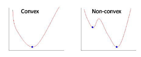 Fig2. Convex and non-convex functions. (image source)
Instead of Mean Squared Error, we use a cost function called Cross-entropy (or Log Loss). The cross-entropy cost functions can be divided into two functions: one for $y=0$ and one for $y=1$.
Training data: $D = \{<x^1,y^1>,\cdots,<x^m,y^m>\}$
Every instance has $n+1$ features. $x=<x_0,\cdots,x_n>$, where $x_0=1$
$w$ is the vector of parameters: $w=<w_0,\cdots,w_n>$
And, $h_{w}(x) = P(y=1|x,w)=\dfrac{1}{1+e^{-wx}}$
The cost functions for each data point $i$ are:
- $J_{y=1}^i(w)=-\log(h_{w}(x^i))$ if $y=1$
- $J_{y=0}^i(w)=-\log(1-h_{w}(x^i))$ if $y=0$
Note: The benefit of taking the logarithm is that these smooth monotonic functions (i.e. always increasing or always decreasing functions) make it easy to calculate the gradient and minimize cost.
We can interpret cost functions as follows:
- if $y=1$:
- if $h_w(x)=0$ and $y=1$, cost is very large (infinite)
- if $h_w(x)=1$ and $y=1$, cost $=0$
 Fig3. cost function $-log(h(x))$ vs $h(x)$ when y=1
- if $y=0$:
- if $h_w(x)=1$ and $y=0$, cost is very large (infinite)
- if $h_w(x)=0$ and $y=0$, cost $=0$
- if $h_w(x)=1$ and $y=0$, cost is very large (infinite)
 Fig4. cost function $-log(1-h(x))$ vs $h(x)$ when y=0
The two cost functions can be combined into a single function:
$$J(w)=-\frac{1}{m}\sum_{i=1}^{m}\left[y^i\log(h_{w}(x^i))+(1-y^i)\log(1-h_{w}(x^i))\right]$$
If we take the derivative of the cost function $J(w)$, we have:
$$\frac{\partial J(w)}{\partial w_j}=\sum_{i=1}^{m}x_j^i\left(y^i-h_w(x^i)\right)$$
which is the same function we obtained by taking the derivative of expression while computing MLCE.
Example: Predict whether a student will pass or fail an exam
We are given a dataset on students exam results and we would like to predict whether a student will pass or fail based on the number of hours and the amount of sleep they had.
Implemented Functions
All the functions, their implementations and documentations are described below. Some of functions are adopted from here.
# Read the training set file and create a data object
file_name = os.path.join("data","data_logregression.csv")
data = load_data(file_name)
data
Feature vector $x=[x_0,x_1,x_2]$ where $x_0=1, x_1="studied", x_2="slept"$. The labels are $y=\{0,1\}$ and parameters include $w=[w_0,w_1,w_2]$
$P(y=1|x,w)=\frac{1}{1+e^{-z}}$ where $z=w_0+w_1x_1+w_2x_2$
Let's represent the data with scatter plot.
# Display the scatter chart of the training data
plot_data(data)
We initialize the variables before start training (i.e. fitting the paramaters).
# emprical value. Experiment with different learning rates.
learning_rate = 0.1

# x_0, x_1, x_2 where x_0 = 1
num_features = 3

# w_0, w_1, w_2
parameters = np.zeros((num_features,1))
iterations = 3000

# number of training examples
num_examples = len(data)

# class labels (i.e. passed/failed) of the training examples
labels = np.array(data["passed"]).reshape(100,1)

# matrix of (examples, features)
x = np.ones((num_examples,1))
examples = np.array(data[["studied","slept"]])
x  = np.append(x,examples, axis=1)

# Fit the model
parameters, cost_history = train(x,labels,parameters,learning_rate,iterations)

print("w = {}".format(parameters))

# Compute the accuracy i.e. total number of correctly predicted labels
# divide by total number of predictions
predictions = predict(x,parameters)
predicted_labels = classify(predictions)
accuracy = get_accuracy(predicted_labels,labels)
print("accuracy = {}".format(accuracy))
# prepare the data to plot cost vs. iterations
xx = np.arange(0,iterations)
yy = np.array(cost_history)
source = pd.DataFrame({"x":xx, "y":yy})

# plot the cost vs. iterations chart
alt.Chart(source).mark_line(size=3,color="red").encode(
    alt.X("x",title="Iterations"),
    alt.Y("y",title="cost",scale=alt.Scale(domain=[0.2,0.7]))
)
Plot the Decision Boundary
We also can plot the decision boundary and see how two classes (passed/failed) are separated. The decision boundary equation is $w_0+w_1x_1+w_2x_2=0$. Therefore, we predict $y=1$ if $w_0+w_1x_1+w_2x_2\geq 0$, otherwise we predict $y=0$. Considering our example, the decision boundary is a line with equation: $$x_2 = -\frac{w_0}{w_2}-\frac{w_1}{w_2}x_1$$
(w_0,w_1,w_2) = parameters
x_points = np.linspace(0,10,100)

# decision boundary line rule
decision_boundary_line = -(w_1/w_2) * x_points -(w_0 / w_2)

source = pd.DataFrame({"x":x_points, "y":decision_boundary_line})
db_chart = alt.Chart(source).mark_line(size=3,color="red").encode(
    alt.X("x",title="studied"),
    alt.Y("y",title="slept",scale=alt.Scale(domain=[-2,10]))
)
data_chart = plot_data(data)

# plot the training data and the decision boundary line
data_chart + db_chart
Multi-class Logistic Regression
If we have $K$ classes, $y=\{0,1,\cdots,K-1\}$ instead of two, $y=\{0,1\}$, we can expand our binary logistic regression into a multiclass classification. There are two approaches for multiclass logistic regression:
1- One versus all:
- We train $K$ binary logistic regression classifier for each class, and choose the class with the biggest probability (i.e. most likely class).
2- Softmax:
- Softmax is a function that takes as input a vector of $K$ real numbers, and normalizes it into a probability distribution consisting of $K$ probabilities proportional to the exponentials of the input numbers. Thus, the predicted probability for the $i'th$ class given a sample vector $x$ and a weighting vector $w$ is:
$$P(y=i|x,w) = \dfrac{e^{w^Tx}}{\sum_{i=1}^{K}e^{w_i^Tx}}$$
How to deal with categorical (discrete) input features?
The input features often include numeric (continuous) as well as categorical (discrete) features. For instance, salary, age, price, etc. are numeric features and gender (male/female), country of birth (e.g. US, Australia, ...), color (e.g. yellow, blue,...) and zip codes (10005, 98360,...) are categorical features. Therefore, the questions becomes: How to multiply categorical features by coefficients?
When we have categorical input features, we must convert them into numeric features. One common way to encode categories as numeric features is via one-hot encoding.
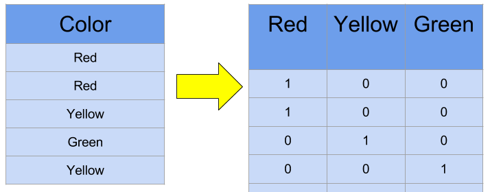 Fig5. One-hot encoding. [Image Source]
References
[1] Tom Mitchell. Naive Bayes and Logistic Regression
[2] Machine Learning Glossary. Logistic Regression