What is Naive Bayes Method?
Naive Bayes technique is a supervised method. It is a probabilistic learning method for classifying documents particularly text documents. It works based on the Naive Bayes assumption. Navie Bayes assumes that features $x_1, x_2, \cdots, x_n$ are conditionally independent given the class labels $y$. In other words:
$$P(x_1,x_2,\cdots,x_n|y)=P(x_1|y)P(x_2|y)\cdots P(x_n|y)=\prod_{i=1}^{n}P(x_i|y)$$
Although often times $x_i$'s are not really conditionally independent in real world, nevertheless, the approach performs surprisingly well in practice, particularly document classification and spam filtering.
Naive Bayes (NB) for Text Classification
Let $D$ be a corpus of documents where each document $d$ is represented by a bag of words (i.e. the order of words does not matter), and has a label $y_d$. If the total number of labels are two $y=\{0,1\}$, meaning that every document belongs to the class 0 or 1, then the problem is a binary classification. Otherwise it is called a multi-class classification, $y=\{0,1, \cdots, k\}$. For instance, for sentiment analysis we have two classes: "positive" and "negative", therefore, $y=\{0,1\}$, 0 representing "negative" class and 1 representing "positive" class, respectively.
The words of the documents are the features and the total number of features is the size of the vocabulary $|v|$ (i.e. total number of unique words in the corpus). For classifying documents, first we represent each document $d$ as a vector of the words $d=<x_{1}, x_{2},\cdots,x_{v}>$. Then the probability of document $d$ being in class $y=c$ is:
$$P(y=c|x_1,x_2,\cdots,x_v)=\dfrac{P(y=c)P(x_1,x_2,\cdots,x_v|y=c)}{P(x_1,x_2,\cdots,x_v)}$$
Assuming conditional independence between $x_i$'s:
$$P(y=c|x_1,x_2,\cdots,x_v)=\dfrac{P(y=c)\prod_{i=1}^{|v|}P(x_i|y=c)}{P(x_1,x_2,\cdots,x_v)}$$
We can drop the denominator as it is a normalization constant. Thus we have:
$$P(y=c|x_1,x_2,\cdots,x_v)\propto P(y=c)\prod_{i=1}^{|v|}P(x_i|y=c)$$
In text classification, our goal is to find the best class for the document $d$. The best class in NB classification is the most likely or maximum a posteriori (MAP) class $y^{map}$. Therefore:
$$y^{map} =\underset{y}{\arg\max}\quad P(y=y_k)\prod_i^{|v|} P(x_i|y=y_k)$$
How to Estimate Parameters $p(y)$ and $p(x_i|y)$
In the context of text classification, to estimate the parameters $P(y)$ and $P(x_i|y)$ we use relative frequency, which assigns the most likely value of each parameter given the training data. For estimating the prior:
$$\hat{P}(y=c)=\dfrac{N_c}{|D|}$$
where $N_c$ is the total number of documents with label $c$ and $|D|$ is total number of documents in the corpus $D$.
We estimate the conditional probability $\hat{P}(x_i|y=c)$ as the relative frequency of term $x_i$ in documents belonging to class $c$:
$$\hat{P}(x_i=t|y=c)=\dfrac{N_{ct} + \alpha}{\sum_{t'=1}^v (N_{ct'}+\alpha)}=\dfrac{N_{ct} + \alpha}{\sum_{t'=1}^v N_{ct'}+\alpha|v|}$$
where $N_{ct}$ is the number of occurrences of $t$ (i.e. count or frequency of $t$) in training documents from class $c$, and $\sum_{t'=1}^v N_{ct'}$ is total count of all the words in documents with label $c$. The parameter $\alpha \geq 0$ is called the smoothing prior. You can think of it as "virtual" or "imaginary" counts, which prevents the probabilities from becomming zero when a feature does not exist in the training data. When $\alpha =1$, it is called Laplace smoothing.
Toy Example
Let's assume that we have a small dataset shown below: (example is adopted from here)
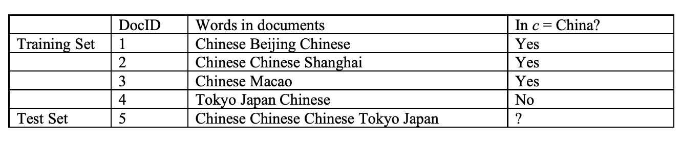
According to this dataset, we want to classify the test document. The vocabulary has 6 words: {"Chinese", "Tokyo", "Japan", "Beijing", "Shanghai", "Macao"}. Therefore, each document is a vector of these words. For example, document $d_1 = <2,0,0,1,0,0>$. Now, the first step to classify the test document $d_5$ is to calculate the priors:
$\hat{P}(y=yes)=\frac{3}{4}$ and $\hat{P}(y=no)=\frac{1}{4}$. Then, we compute the conditional probabilities, assuming $\alpha=1$:
$$\hat{P}(Chinese|y=yes)=\dfrac{5+1}{8+6}=\dfrac{6}{14}=\dfrac{3}{7}$$
$$\hat{P}(Tokyo|y=yes)=\hat{P}(Japan|y=yes)=\dfrac{0+1}{8+6}=\dfrac{1}{14}$$
$$\hat{P}(Chinese|y=no)=\dfrac{1+1}{3+6}=\dfrac{2}{9}$$
$$\hat{P}(Tokyo|y=yes)=\hat{P}(Japan|y=yes)=\dfrac{1+1}{3+6}=\dfrac{2}{9}$$
We then get,
$$\hat{P}(y=yes|d_5)\propto 3/4 \cdot (3/7)^3 \cdot 1/14 \cdot 1/14 \approx 0.0003$$
$$\hat{P}(y=no|d_5)\propto 1/4 \cdot (2/9)^3 \cdot 2/9 \cdot 2/9 \approx 0.0001$$
Thus, the classifier assigns the test document to $c=$ China. The reason for this classification decision is that the three occurrences of the positive indicator Chinese in $d_5$ outweigh the occurrences of the two negative indicators Japan and Tokyo.
Implementation
For sentiment classification, I used the popular IMDB dataset from here. This dataset provides a set of 25,000 highly polar movie reviews for training, and 25,000 for testing.
First, we read the files and create our training and test sets.
print('Loading training data...')
train_data = load_data('train')
print('done!')
print('Loading test data...')
test_data  = load_data('test')
print('done!')
# Unpack the (text, label) for training and test data
x_train, y_train = zip(*train_data)
x_test, y_test   = zip(*test_data)
There are many different configurations that we can experiment with. To start it off, we train the model based on input arquments. This model removes the stop words, creates the unigrams and bigrams for all the documents and take into account the entire vocabulary. After training, the model outputs useful information such as the accuracy of the model and total training time.
# Training the model with following parameters
# Remove stop words
stop_words   = 'english'

# Consider uni-grams and bi-grams
ngram_range  = (1, 2)

# Take all the features into account
max_features = None

preds, acc = run(x_train, y_train, x_test, y_test, stop_words, ngram_range, max_features)
In the this experiment, we only consider the unigrams (i.e. representing documents based on terms). The remaining input parameters are as before. We can see that the accuracy is decreased, which indicate that bigrams help the classification task.
# Another configuration
stop_words   = 'english'
ngram_range  = (1, 1)
max_features = None
preds, acc = run(x_train, y_train, x_test, y_test, stop_words, ngram_range, max_features)
In this configuration, we only consider the 5000 common words in the documents, but take the bigrams into account and perform the classification task. It gives better accuracy comparing with previous experiment.
# Another configuration
stop_words   = 'english'
ngram_range  = (1, 2)
max_features = 5000
preds, acc = run(x_train, y_train, x_test, y_test, stop_words, ngram_range, max_features)
In this experiment, we keep the stop words but limit the vocabulary size to 5000 and only consider unigrams. The result shows that cutting the size of the vocab lowers the accuracy.
# Another configuration
stop_words   = None
ngram_range  = (1, 1)
max_features = 5000
preds, acc = run(x_train, y_train, x_test, y_test, stop_words, ngram_range, max_features)
In the last experiment, we keep the stop words, consider both unigrams and bigrams and take into account the entire vocabulary. It gives us the best accuracy among all the configuration we experimented with. It demonstrates that keeping stop words help in better sentiment analysis, unlike some other classification tasks.
# Another configuration
stop_words   = None
ngram_range  = (1, 2)
max_features = None
preds, acc = run(x_train, y_train, x_test, y_test, stop_words, ngram_range, max_features)
There are other configurations that I did not experiment with. But I leave that as an exercise. ;)
Training an LSTM model on the IMDB sentiment classification task
The code below is adopted directly from Keras website. This code implements an LSTM model on the same IMDB dataset for sentiment analysis task.
from tensorflow.keras.preprocessing import sequence
from tensorflow.keras.models import Sequential
from tensorflow.keras.layers import Dense, Embedding
from tensorflow.keras.layers import LSTM
from tensorflow.keras.datasets import imdb

max_features = 20000
# cut texts after this number of words (among top max_features most common words)
maxlen = 80
batch_size = 32

print('Loading data...')
(x_train, y_train), (x_test, y_test) = imdb.load_data(num_words=max_features)
print(len(x_train), 'train sequences')
print(len(x_test), 'test sequences')

print('Pad sequences (samples x time)')
x_train = sequence.pad_sequences(x_train, maxlen=maxlen)
x_test = sequence.pad_sequences(x_test, maxlen=maxlen)
print('x_train shape:', x_train.shape)
print('x_test shape:', x_test.shape)

print('Build model...')
model = Sequential()
model.add(Embedding(max_features, 128))
model.add(LSTM(128, dropout=0.2, recurrent_dropout=0.2))
model.add(Dense(1, activation='sigmoid'))

# try using different optimizers and different optimizer configs
model.compile(loss='binary_crossentropy',
              optimizer='adam',
              metrics=['accuracy'])

print('Train...')
model.fit(x_train, y_train,
          batch_size=batch_size,
          epochs=15,
          validation_data=(x_test, y_test))
score, acc = model.evaluate(x_test, y_test,
                            batch_size=batch_size)
print('Test score:', score)
print('Test accuracy:', acc)
It takes a lot of time to run on CPU, therefore I ran it on Google Colab, which took roughly around 30 minutes to train. You can see the result below:
Loading data...
25000 train sequences
25000 test sequences
Pad sequences (samples x time)
x_train shape: (25000, 80)
x_test shape: (25000, 80)
Build model...
Train...
Train on 25000 samples, validate on 25000 samples
Epoch 1/15
25000/25000 [==============================] - 137s 5ms/sample - loss: 0.4546 - accuracy: 0.7889 - val_loss: 0.3738 - val_accuracy: 0.8394
Epoch 2/15
25000/25000 [==============================] - 133s 5ms/sample - loss: 0.2930 - accuracy: 0.8816 - val_loss: 0.3865 - val_accuracy: 0.8281
Epoch 3/15
25000/25000 [==============================] - 130s 5ms/sample - loss: 0.2111 - accuracy: 0.9173 - val_loss: 0.4440 - val_accuracy: 0.8348
Epoch 4/15
25000/25000 [==============================] - 128s 5ms/sample - loss: 0.1484 - accuracy: 0.9449 - val_loss: 0.4976 - val_accuracy: 0.8283
Epoch 5/15
25000/25000 [==============================] - 127s 5ms/sample - loss: 0.1022 - accuracy: 0.9627 - val_loss: 0.6127 - val_accuracy: 0.8238
Epoch 6/15
25000/25000 [==============================] - 126s 5ms/sample - loss: 0.0781 - accuracy: 0.9734 - val_loss: 0.6076 - val_accuracy: 0.8173
Epoch 7/15
25000/25000 [==============================] - 126s 5ms/sample - loss: 0.0587 - accuracy: 0.9794 - val_loss: 0.7733 - val_accuracy: 0.8188
Epoch 8/15
25000/25000 [==============================] - 126s 5ms/sample - loss: 0.0430 - accuracy: 0.9860 - val_loss: 0.9582 - val_accuracy: 0.7603
Epoch 9/15
25000/25000 [==============================] - 125s 5ms/sample - loss: 0.0482 - accuracy: 0.9847 - val_loss: 0.7996 - val_accuracy: 0.8190
Epoch 10/15
25000/25000 [==============================] - 125s 5ms/sample - loss: 0.0270 - accuracy: 0.9916 - val_loss: 0.8270 - val_accuracy: 0.8106
Epoch 11/15
25000/25000 [==============================] - 125s 5ms/sample - loss: 0.0226 - accuracy: 0.9927 - val_loss: 0.8667 - val_accuracy: 0.8120
Epoch 12/15
25000/25000 [==============================] - 126s 5ms/sample - loss: 0.0176 - accuracy: 0.9944 - val_loss: 1.0325 - val_accuracy: 0.8141
Epoch 13/15
25000/25000 [==============================] - 126s 5ms/sample - loss: 0.0149 - accuracy: 0.9948 - val_loss: 0.9852 - val_accuracy: 0.8104
Epoch 14/15
25000/25000 [==============================] - 126s 5ms/sample - loss: 0.0140 - accuracy: 0.9955 - val_loss: 1.0443 - val_accuracy: 0.8127
Epoch 15/15
25000/25000 [==============================] - 125s 5ms/sample - loss: 0.0133 - accuracy: 0.9956 - val_loss: 1.1763 - val_accuracy: 0.8127
25000/25000 [==============================] - 16s 656us/sample - loss: 1.1763 - accuracy: 0.8127
Test score: 1.1762849241028726
Test accuracy: 0.81268
Comparing Naive Bayes with LSTM for Sentiment Analysis
If we compare Naive Bayes with LSTM, we find out some interesting observations:
Implementing Naive Bayes is very straightforward compared to LSTM.
Training NB is extremely fast, a few seconds, whereas the implemented LSTM takes about 30 minutes on GPU. Please note that this LSTM implementation even cuts the max features into 20000.
Number of parameters that we can alter for NB is very few unlike LSTM that we need to perform lots of fine tuning.
Scaling Naive Bayes implementation to large datasets having millions of documents is quite easy whereas for LSTM we certainly need plenty of resources.
If you look at the image below, you notice that the state-of-the-art for sentiment analysis belongs to a technique that utilizes Naive Bayes bag of n-grams. See the paper for all the details. This method gives the best accuracy higher than many purely deep learning methods such as BERT and LSTM+CNN.
Don't get me wrong! I am a big fan of neural networks and deep learning techniques. The point that I am trying to make is that in many cases we may not need very complex methods for our tasks. My approach is always start off with simpler techniques and if they are not satisfactory, then move to more sophisticated ones.
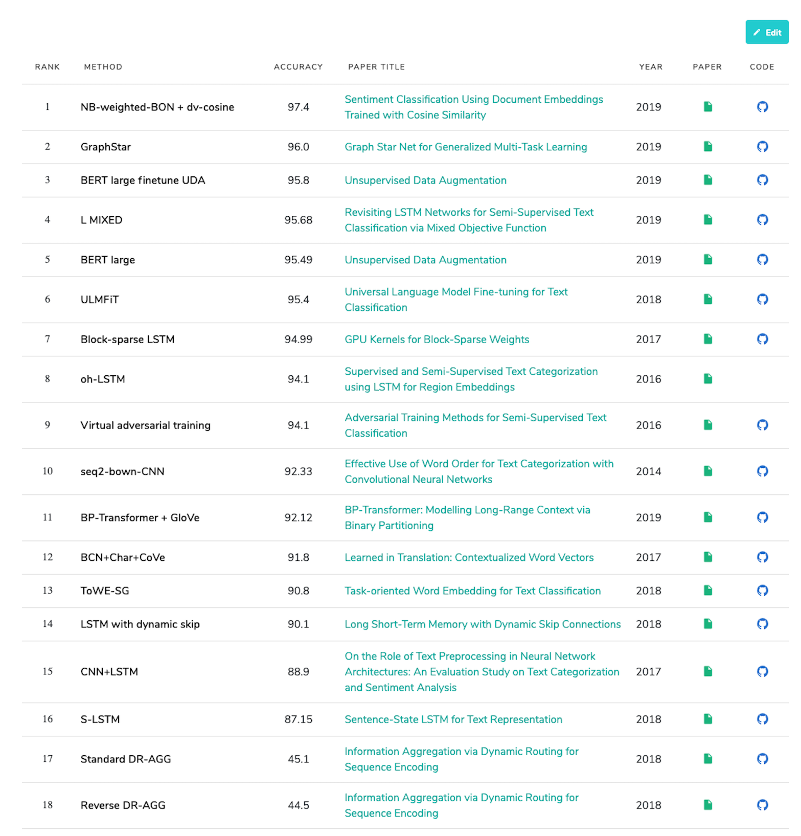 State-of-the-art sentiment analysis on the IMDB dataset. [Image Source]