Definition
Regression is an approach to modeling the relationship between a real-valued target $y$ (dependent variable) and data points $X$ (independent variables). In other words, linear regression describes the relationship between input and output and predicts the output based on the input data.
We wish to learn $f:X\to Y$, where $Y$ is a real number, given $\{<X^1,y^1>,\cdots, <X^m,y^m>\}$.


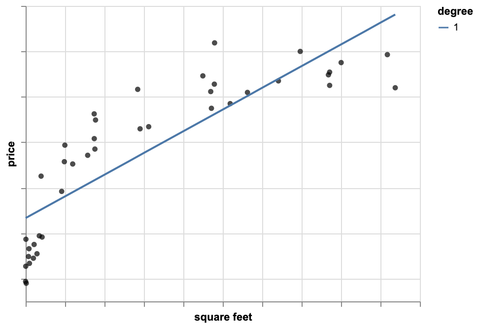
Check the prices of the sold houses that have the same square feet as my house.

What if no house was sold with exactly the same size?
I look at some small range of square footage around my actual square footage, and check the houses within this range.

The problem is, I am only considering a few houses and throwing out all other observations as if they have nothing to do with the value of my house.
We can leverage all the information we can from all the observations to come up with a good prediction.

Formal Problem Description
Let's assume that we are going to predict the price of houses (in dollars), $y$, based on their area (in square feet), $x$. Therefore, training set = $\{<x^1,y^1>,\cdots,<x^m,y^m>\}$, where:
- $m$: number of trainig examples
- $x$: input variable
- $y$: output variable or target label
- $(x^i,y^i)$: is the $i$th training example
$$\hat y = f(x) = w_0 + w_1x$$
where $w_0$ and $w_1$ are the paramaters of the $f(x)$ that we need to find.


import numpy as np
import pandas as pd
import altair as alt
from ipywidgets import *

# Generate some random data
rng = np.random.RandomState(1)
number_of_points = 50
x = rng.rand(number_of_points)**2
y = 10 - 0.5 / (x + 0.1) + rng.randn(number_of_points)
source = pd.DataFrame({"square feet": x, "price": y})

# Define the chart
base = alt.Chart(source).mark_circle(color="blue", size=70).encode(
    alt.X("square feet", axis=alt.Axis(labels=False)),
    alt.Y("price", axis=alt.Axis(labels=False)))
def plot_poly(degree):
    return base + base.transform_regression(
        "square feet", "price", method="poly", order=degree).mark_line(size=3, color="red")
interact(plot_poly,degree=widgets.IntSlider(min=1, max=20, step=1, value=1));
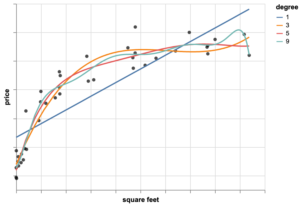
Polynomial Regression Model
If we represent the relationship between the independent variable $x$ and dependent variable $y$ as an $n$th degree polynomial, then the regression model is called polynomial regression. Therefore, we have:
$$y_i=w_0+w_1x_i+w_2x_i^2+\cdots+w_nx_i^n+\epsilon_i$$
We treat each $x_i^p$ for $p=1,\cdots,n$ as a different feature. i.e. $feature\ 1=x, feature\ 2=x^2,\cdots, feature\ n=x^n$.
Overfitting Problem
We fit a quadratic function and look at the plot and notice that quadratic fit is better than a line. Then, we might think a higher order polynomial even fits the data better. We try 13th order polynomial and minimize the residual sum of squares. The residual sum of error is quite small, which means this 13th order polynomial is the best fit for the data. However, based on this function the price my house is unrealistically low whereas I think my house isn't worth so little.

Quadratic function: $\hat{y}=w_0+w_1x+w_2x^2$, and 13th order polynomial: $\hat{y}=w_0+w_1x+w_2x^2+\cdots w_{13}x^{13}$
The reason is this 13th order polynomial is overfitting the data. It means even though our model fits the observations really well, it doesn't generalize well to predicting new observations. It minimizes the residual sum of squares, but it ends up leading to very bad predictions. Although, the quadratic function didn't minimize residual sum of squares as much as the 13th order polynomial, it still is a better model.
How to Prevent Overfitting
Considering our dataset, we remove some of the houses and fit the model on the remaining ones. We minimize the RSS error. Then, we predict the values of the held-out houses (i.e. the houses we left out) and compare the predicted values with their actual values.
The dataset (e.g houses) that we use to fit the model is called Training set. And the dataset that we use for prediction (held-out) is called Test set.
In order to see how well our model works, we do a little bit of analysis. We look at the residual sum of squares on the houses in our training set that is called training error. We then estimate the model parameters $w=[w_0,w_1]$. We take these estimated parameters and see how well we predicting the actual values of the houses that are in test set. We use the predicted value (value on the line) and again we look at the residual sum of squares over all the houses that are in the test set, and is called test error. Then, we assess how the test error and training error vary as function of the model complexity.

If we notice that there is a big difference between training error and test error, it means that model is likely overfitted. Another sign of overfitting is that the parameter values $w$ are very large.
Regularization
We add a penalty term to the Residual sum of squares (RSS). This extra term penalizes the parameters $w$ from getting large values. Therefore, instead of minimizing the RSS, we minimize the combination of RSS and this additional regularization expression.
$$J(\mathbf{w})=\sum_{i=1}^{m}\Big( y_i-f(x_i)\Big)^2+\lambda\|\mathbf{w}\|^2$$
where $\|\mathbf{w}\|^2 = \sqrt{w_1^2 +w_2^2+\cdots w_k^2}$, and $\lambda$ is a hyperparameter that balances tradeoff.
Linear Regression General Expansion
In general, if we have a dataset of $m$ instances with $k$ features, $\mathbf{x}=<x_1,x_2,\cdots,x_k>$ and a real valued target $y$, then the linear regression model takes the form:
$$y_i=w_0+w_1h_1(x_1)+w_2h_2(x_2)+\cdots+w_kh_k(x_k)+\epsilon_i= w_0 +\sum_{j=1}^{k}w_jh_j(x_i)+\epsilon_i$$
Considering our house price prediction, instead of using only area of the house, we can add more features such as number of bathrooms, number of bedrooms, age of the house, etc.
The Regression Problem Statement
The general approach is as follows:
Instances: $<\mathbf{x}_i,y_i>$
Learn: mapping from $\mathbf{x}$ to $y\equiv f(\mathbf{x})$
Given the basis functions $h_1, h_2,\cdots,h_k$ where $h_j(\mathbf{x})\in \mathbb{R}$
Find coeffcients $\mathbf{w}=[w_0,w_1,\cdots,w_k]$, where $f(\mathbf{x})\thickapprox \hat{f}(\mathbf{x})=w_0+\sum_{j}w_jh_j(\mathbf{x})$
- In order to find coefficients, we need to minimize the mean residual square error:
$$J(\mathbf{w}) = \frac{1}{m}\sum_{i=1}^{m}\left( f(\mathbf{x}_i) - \left(w_0 +\sum_{j=1}^{k}w_jh_j(\mathbf{x})\right)\right)^2$$
$$\mathbf{w}^* = \underset{\mathbf{w}}{\arg\min}\ J(\mathbf{w})$$
We would like to find a line that fits our training examples the best.
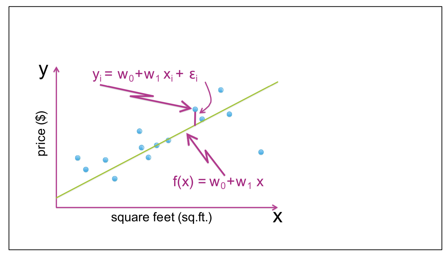
Since we are looling for a line to fit our training set, we need to find a function $\hat y = f(x)$ that estimates $y^i$ for all $1\leq i \leq m$. Thus, we have:
$$\hat y = f(x) = w_0 + w_1x$$
$w_0$ and $w_1$ are the paramaters that we need to find.
Cost Function (Error Function)
We wish to estimate the actual $y$, i.e. we want to minimize the error as much as possible. The error is the difference between the actual $y^i$ and our estimated/predicted $\hat{y}^i$ for all $1\leq i \leq m$.
The error/cost function is:
$$J(w_0,w_1) = \frac{1}{m}\sum_{i=1}^{m}\left( y^i - (w_0 + w_1 x^i)\right)^2$$
Precisely, we need to minimize the mean residual squared error:
$$\text{minimize } J(w_0,w_1) = \underset{w0,w_1}{\arg\min} \frac{1}{m}\sum_{i=1}^{m}\left( \hat{y}^i - (w_0 + w_1 x^i)\right)^2$$
Fitting the Linear Regression Model using Gradient Descent Algorithm
In order to mininze the cost function, we need to take the gradient (i.e. derivative) of the function with resptect to our parameters $w_0$ and $w_1$, set it zero and solve for $w_0$ and $w_1$.
$$\frac{\partial{J}}{\partial{w_0}} = \frac{-2}{m} \sum_{i=1}^{m}\left(\hat{y}^i - (w_0 + w_1 x^i)\right)$$
$$\frac{\partial{J}}{\partial{w_1}} = \frac{-2}{m} \sum_{i=1}^{m}x^i\left(\hat{y}^i - (w_0 + w_1 x^i)\right)$$
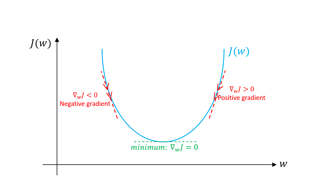
image source: https://towardsdatascience.com/gradient-descent-algorithm-and-its-variants-10f652806a3
The gradient descent algorithm:
initialize $w_0^{(0)} = w_1^{(0)} = 0$, for $t=0$
for $t=1$ to num_iterations
$w_0^{(t+1)} = w_0^{(t)} - \eta \frac{-2}{m} \sum_{i=1}^{m}\left(\hat{y}^i - (w_0 + w_1 x^i)\right) $
$w_1^{(t+1)} = w_1^{(t)} - \eta\frac{-2}{m} \sum_{i=1}^{m}x^i\left(\hat{y}^i - (w_0 + w_1 x^i)\right)$
$t = t+1$
Run an Example
In this example, we generate some linear-looking data and then find the line that fits the data. The function that we use to generate the data is $y=5+3x+\text{Gaussian noise}$. Our goal is to find $\theta=[w_0,w_1]$ where $w_0=5$ and $w_1=3$ or close enough, as we have noise and it makes it impossible to recover the exact paratmeters of the function. We use the generate_data function to generate the training data.
np.random.seed(100)

# Approximate y = 5 + 3x
X,y = generate_data(100)
The chart below shows the generated dataset.
origin_chart = make_point_plot(X,y)

#show the chart
origin_chart
We set the initial parameters to 0: $w_0^{(0)} = w_1^{(0)} = 0$, define the number of iterations of the graditent descent algorithm as well as the learning rate. Then, we run the gradient_descent function. The outputs of this function are the estimated parameters $w_0$ and $w_1$.
initial_w_0 = 0
initial_w_1 = 0
num_iterations = 1000
learning_rate = 0.1

data = (X,y)
w_0,w_1 = gradient_descent(data,initial_w_0,initial_w_1,learning_rate,num_iterations)

print("w_0 = {}, w_1 = {}".format(w_0,w_1))
The estimated parameters are $w_0 = 4.923$ and $w_1 = 2.97$ that are close enough to $w_0=5$ and $w_1=3$. Let's plot the line.
y_predicted = w_0 + w_1 * X
line = make_line_plot(X,y_predicted)

#show the charts
origin_chart + line
num_iterations = 1000
l_rates = [0.001,0.01,0.1,0.002]
all_params = []

# X,y = generate_data()
data = (X,y)
for i in range(0,len(l_rates)):
    initial_w_0 = 0
    initial_w_1 = 0
    learning_rate = l_rates[i]
    w_0,w_1 = gradient_descent(data,initial_w_0,initial_w_1,learning_rate,num_iterations)
    all_params.append((w_0,w_1))
    print("learning_rate: {:.4f} => w_0 = {}, w_1 = {}".format(learning_rate,w_0,w_1))
Graduate Admission Prediction
We are going to use a dataset to predict the chance of getting admission in graduate school from the perspective of Indian students. The dataset is available at this link.
Content
The dataset contains several parameters which are considered important during the application for Masters Programs. The parameters included are :
GRE Scores ( out of 340 )
TOEFL Scores ( out of 120 )
University Rating ( out of 5 )
Statement of Purpose and Letter of Recommendation Strength ( out of 5 )
Undergraduate GPA ( out of 10 )
Research Experience ( either 0 or 1 )
Chance of Admit ( ranging from 0 to 1 )
Let's code it up!
We are using Turi Create library.
import turicreate as tc
import os


# Load the data
file_name = os.path.join("data","admission_predict.csv")
data = tc.SFrame(file_name)
# Split the data into train and test sets
train_data, test_data = data.random_split(0.8)
# Create the model and automatically pick the right model for the data
model = tc.linear_regression.create(train_data, target="Chance of Admit",
                                                features=["GRE Score","TOEFL Score","University Rating","SOP","LOR" ,"CGPA","Research"])
model.coefficients
# Do the prediction and save them into an array
predictions = model.predict(test_data)
# Evaluate the model and save the results
results = model.evaluate(test_data)
results